This is the whole pipeline on one cohort, in the order it has to run: say what is being predicted, account for every row that leaves, describe what is left, fit, validate on a stated basis, and draw an instrument that is checked against the model rather than assumed to match it.
Every number below comes from synthetic data. The package carries no
patient data and never will, so mm_synthetic_cohort() is
what the examples, the fixtures and the articles all run on.
A cohort with known truth
raw <- mm_synthetic_cohort(n = 500, prevalence = 0.11, seed = 1978)
str(raw, give.attr = FALSE)
#> 'data.frame':    500 obs. of  8 variables:
#>  $ age       : num  48.7 67.1 54.7 94 73.2 48.3 43.4 64.8 57.5 39.9 ...
#>  $ bmi       : num  24.3 18.2 32.2 21.3 36.3 29.9 18.1 20.7 37 19.1 ...
#>  $ sex       : Factor w/ 2 levels "female","male": 1 1 1 1 1 1 1 2 1 1 ...
#>  $ prior_uti : Factor w/ 2 levels "no","yes": 1 1 1 2 1 1 1 1 1 1 ...
#>  $ indication: Factor w/ 3 levels "incontinence",..: 1 3 1 3 1 2 1 1 1 3 ...
#>  $ year      : int  2024 2020 2019 2023 2023 2020 2024 2022 2024 2021 ...
#>  $ pid       : chr  "p0179" "p0008" "p0079" "p0013" ...
#>  $ event     : int  0 0 0 0 0 0 0 0 0 0 ...
attr(raw, "truth")$formula
#> [1] "event ~ 0.0011*(age-62)^2 + 0.045*(bmi-29) + 0.35*male + 0.80*prior_uti + 0.60*prior_uti:male"
The generating model is deliberately not additive. It carries a
quadratic age effect and one prior_uti by sex
interaction, because a pipeline exercised only on additive data never
reveals whether its spline and hierarchy handling are right. The
truth attribute is what later sections are checked
against.
About 8% of rows are a second visit by a patient already present,
which is what pid is for:
sum(duplicated(raw$pid))
#> [1] 40
The generator produces complete data and a real export does not, so a little missingness goes in deliberately. Everything downstream has to cope with it, and a vignette on complete data would not show whether it does.
Describe what was exported, before deciding who is eligible
desc <- mm_eda(raw, by = "event",
               vars = c("age", "bmi", "sex", "prior_uti", "indication"))
desc$table
#>         variable           statistic           Overall         event = 0
#> 1  (denominator)                   n               500               448
#> 2            age           mean (SD)       62.7 (12.4)       62.3 (12.3)
#> 3            age   median (p25, p75) 63.3 (54.2, 71.3) 63.0 (53.9, 70.5)
#> 4            age      missing, n (%)          0 (0.0%)          0 (0.0%)
#> 5            bmi           mean (SD)        29.3 (5.8)        29.2 (5.7)
#> 6            bmi   median (p25, p75) 29.1 (25.3, 33.0) 29.0 (25.3, 32.7)
#> 7            bmi      missing, n (%)          9 (1.8%)          8 (1.8%)
#> 8            sex       female, n (%)       356 (71.2%)       326 (72.8%)
#> 9            sex         male, n (%)       144 (28.8%)       122 (27.2%)
#> 10           sex      missing, n (%)          0 (0.0%)          0 (0.0%)
#> 11     prior_uti           no, n (%)       357 (71.4%)       332 (74.1%)
#> 12     prior_uti          yes, n (%)       143 (28.6%)       116 (25.9%)
#> 13     prior_uti      missing, n (%)          0 (0.0%)          0 (0.0%)
#> 14    indication incontinence, n (%)       232 (47.0%)       203 (45.9%)
#> 15    indication     prolapse, n (%)       106 (21.5%)        96 (21.7%)
#> 16    indication    retention, n (%)       156 (31.6%)       143 (32.4%)
#> 17    indication      missing, n (%)          6 (1.2%)          6 (1.3%)
#>            event = 1
#> 1                 52
#> 2        66.5 (12.7)
#> 3  66.0 (57.5, 75.6)
#> 4           0 (0.0%)
#> 5         30.5 (6.5)
#> 6  30.5 (25.0, 35.5)
#> 7           1 (1.9%)
#> 8         30 (57.7%)
#> 9         22 (42.3%)
#> 10          0 (0.0%)
#> 11        25 (48.1%)
#> 12        27 (51.9%)
#> 13          0 (0.0%)
#> 14        29 (55.8%)
#> 15        10 (19.2%)
#> 16        13 (25.0%)
#> 17          0 (0.0%)
The missing count sits beside each variable rather than in a separate table, because a percentage whose denominator quietly excludes missing rows reads as a fact about the cohort when it is a fact about the rows that happened to be complete. The denominator each percentage was taken over is the first row.
desc$missing
#>     variable n_missing pct_missing
#> 2        bmi         9         1.8
#> 5 indication         6         1.2
#> 1        age         0         0.0
#> 3        sex         0         0.0
#> 4  prior_uti         0         0.0
desc$duplicates
#> [1] 0
This is a data frame, not a rendered table. gt,
gtsummary, knitr::kable() and Quarto can all
render it, and none of them is needed to compute it.
The cells are strings because the formatting is part of the contract: counts with thousands separators, percentages to one decimal, means with standard deviations, medians with the quartiles. The same four helpers build every cell, so a table cannot be internally inconsistent about how it rounds:
c(mysterymodel:::mm_count(12345),
  mysterymodel:::mm_n_pct(45, 404),
  mysterymodel:::mm_mean_sd(raw$age),
  mysterymodel:::mm_median_iqr(raw$age))
#> [1] "12,345"            "45 (11.1%)"        "62.7 (12.4)"
#> [4] "63.3 (54.2, 71.3)"
Eligibility, with a ledger that reconciles
Each rule is a named one-sided formula. The name is what a flow diagram will say, so it should read as the criterion it expresses.
cohort <- mm_clean(raw, rules = list(
  "aged 40 or over"     = ~ age >= 40,
  "plausible BMI"       = ~ bmi >= 16 & bmi <= 55,
  "indication recorded" = ~ !is.na(indication)
), label = "urodynamics studies as exported")

cohort
#> <mm_cohort>  500 in, 470 out, 30 excluded
#>      500  urodynamics studies as exported
#>      -13  aged 40 or over (did not meet the criterion)
#>      487  remaining
#>       -3  plausible BMI (did not meet the criterion)
#>      484  remaining
#>       -9  plausible BMI (criterion could not be determined for these rows)
#>      475  remaining
#>       -5  indication recorded (did not meet the criterion)
#>      470  remaining
Rows in must equal rows out plus every exclusion.
mm_clean() errors rather than returning a cohort it cannot
reconcile, which is the one thing it exists to prevent:
cohort$ledger[, c("rule", "n_excluded", "n_after", "reason")]
#>                              rule n_excluded n_after
#> 1 urodynamics studies as exported         NA     500
#> 2                 aged 40 or over         13     487
#> 3                   plausible BMI          3     484
#> 4                   plausible BMI          9     475
#> 5             indication recorded          5     470
#>                                             reason
#> 1                                  starting cohort
#> 2                       did not meet the criterion
#> 3                       did not meet the criterion
#> 4 criterion could not be determined for these rows
#> 5                       did not meet the criterion
c(in_ = cohort$n_in, out = cohort$n_out, excluded = cohort$n_excluded)
#>      in_      out excluded
#>      500      470       30
Look at the two plausible BMI lines. Nine rows have no
BMI, so the rule is neither true nor false for them, and they leave
under their own heading rather than passing. A rule that evaluates to
NA is not a pass: treating unknown eligibility as eligible
and treating it as ineligible are different studies, and the difference
belongs in the diagram.
The cohort that goes on to be modelled is complete by construction, because the rules above made completeness a stated eligibility criterion rather than a side effect of whatever the fitting function drops:
mm_eda(cohort, vars = c("age", "bmi", "sex", "prior_uti",
                        "indication"))$missing
#>     variable n_missing pct_missing
#> 1        age         0           0
#> 2        bmi         0           0
#> 3        sex         0           0
#> 4  prior_uti         0           0
#> 5 indication         0           0
Imputation instead of exclusion is a v0.3 item. Until it exists, the exclusion is visible in the ledger, which is the honest version of the same decision.
Skipping the rule does not get you a larger study. rms
drops a row with a missing model variable before fitting, so the rows
would leave anyway, just without appearing anywhere.
mm_model() warns when that happens, names the variable that
cost them, and counts from the fit rather than from the frame it was
handed, because a sample-size gate given rows the model never saw is
lenient in exactly the case that most needs it strict.
The plan, written down before anything is fitted
project <- mm_project(
  slug           = "uds",
  outcome        = "event",
  predictors     = c("age", "bmi", "sex", "prior_uti", "indication"),
  positive_class = 1,
  cohort         = cohort$data,
  split_var      = "year",
  split_at       = 2023,
  cluster_id     = "pid",
  seed           = 1978
)

project
#> <mm_project: uds>
#>   outcome    event (event = 1)
#>   predictors 5: age, bmi, sex, prior_uti, indication
#>   split      year < 2023 develops, the rest is held out
#>   cluster    pid
#>   shape      every continuous predictor linear
#>   seed       1978
Nothing is fitted here. The point of the object is that a reviewer can check it against the protocol instead of reconstructing it afterwards from whichever code ran. It fails closed on configurations that cannot be meant:
mm_project("uds", "event", c("age", "event"))
#> Error:
#> ! `outcome` (event) is also in `predictors`. A model given its own outcome reports perfect discrimination.

mm_project("uds", "event", c("age", "bmi"), split_var = "year")
#> Error:
#> ! `split_var` and `split_at` go together. Temporal validation without a time field does not describe a split.

mm_project("uds", "event", c("age", "bmi"),
           positive_class = "yes", cohort = cohort$data)
#> Error:
#> ! `positive_class` (yes) is not an observed value of `event`. Observed: 0, 1. An inverted positive class inverts every reported risk.
The third is worth dwelling on. An inverted positive class inverts every risk the model goes on to report, and nothing downstream looks wrong.
Fit
model <- mm_model(project, cohort$data,
                  nonlinear    = "age",
                  interactions = list(c("prior_uti", "sex")),
                  knots        = 4)
#> Warning: the development sample may be too small for this model: 317 rows is
#> 663 short of the 980 a model of 9 parameter(s) needs at 10.1% prevalence for
#> 90% shrinkage. Coefficients from a sample this size are expected to be
#> overfitted; see the adequacy element of the returned object.

model
#> <mm_model: uds>
#>   formula    .mm_y ~ rms::rcs(age, 4) + bmi + sex + prior_uti + indication +     prior_uti:sex
#>   developed  317 rows, 32 events
#>   held out   153 rows
#>   parameters 9 non-intercept, 663 short of the sample they need
#>   apparent C 0.7553
#>   fingerprint 7855ae820d29b8c6
The warning is the sample-size gate, and it is the honest answer for
a cohort this size. The gate is the Riley requirement from
pmsampsize, not the events-per-parameter rule, which is
reported as description and labelled as such:
model$adequacy
#> <mm_adequacy>  adequate: FALSE
#>   development 317 rows, 32 events (10.1%)
#>   parameters  9 non-intercept, 3.6 events each (description, not the criterion)
#>   shrinkage   0.655 expected, heuristic
#>   requires    980 rows, 99 events (Riley, from the fitted R2 of 0.164)
#>   317 rows is 663 short of the 980 a model of 9 parameter(s) needs at 10.1% prevalence for 90% shrinkage
Two independent routes agree. The heuristic shrinkage above is computed from the likelihood ratio and the parameter count; the bootstrap calibration slopes in the validation section below are estimated by resampling. The two land within a few hundredths of each other, and neither calculation knows about the other.
Strong hierarchy is enforced before a formula exists, because a formula is the last place to find out:
mm_model(mm_project("uds", "event", c("age", "sex")), cohort$data,
         interactions = list(c("sex", "prior_uti")))
#> Error:
#> ! interaction sex:prior_uti needs its main effect(s) prior_uti among the predictors. An interaction without its main effects is not interpretable.
What was fitted, and what a deployed prediction is allowed to receive:
deparse1(model$formula)
#> [1] ".mm_y ~ rms::rcs(age, 4) + bmi + sex + prior_uti + indication + prior_uti:sex"
model$schema$predictors$sex
#> $type
#> [1] "categorical"
#>
#> $levels
#> [1] "female" "male"
model$schema$predictors$age
#> $type
#> [1] "numeric"
#>
#> $range
#> [1] 40.2 95.0
model$fingerprint
#> [1] "7855ae820d29b8c6ec468b1c8bac2f12128226a11b96a987c765886a9ccae54f"
Preventing outcome leakage in clinical prediction models
A predictor that carries the outcome is not predicting it. The model that results reports near-perfect discrimination, which reads as success, so this is the one mistake in the whole pipeline that makes its own output look better rather than worse.
mm_project() checks that the outcome is not among the
predictors. That is a comparison of names, and a copy under another name
passes it:
leaky <- cohort$data
leaky$triage_flag <- leaky$event        # the outcome, renamed
mm_model(
  mm_project("uds", "event", c("age", "bmi", "triage_flag"),
             positive_class = 1, cohort = leaky, seed = 1978),
  leaky)
#> Error:
#> ! outcome leakage: predictor `triage_flag` reads as binary with 1 is the event, and reproduces the outcome on every one of the 470 compared row(s). A predictor carrying `event` is not predicting it, and a model given one reports near-perfect discrimination, which reads as success. Remove it before fitting.
The detection is on values, not names. A column is read as 0/1 only where that is unambiguous: numeric holding just 0 and 1, a logical, or any column with exactly two observed values. For a two-valued column both assignments are tried, because the labels carry no information:
mysterymodel:::mm_binary_forms(factor(c("yes", "no", "yes")))
#> [[1]]
#> [[1]]$code
#> [1] 0 1 0
#>
#> [[1]]$label
#> [1] "\"no\" is the event"
#>
#>
#> [[2]]
#> [[2]]$code
#> [1] 1 0 1
#>
#> [[2]]$label
#> [1] "\"yes\" is the event"
mysterymodel:::mm_binary_forms(c("mild", "moderate", "severe"))
#> list()
Five things that are not the same
A direct copy of the outcome is settled by arithmetic. There is no cohort in which a column reproducing the outcome on every row is a prediction, so it is refused.
Perfect separation is not. Every observed level of a categorical predictor sitting in one outcome class, or a numeric threshold that divides the classes completely, can be leakage and can equally be a cohort with four events. It is reported for you to settle, and the model still fits:
rare <- data.frame(event = c(rep(0L, 96), rep(1L, 4)),
                   age = cohort$data$age[1:100])
rare$marker <- c(runif(96, 0, 1), runif(4, 5, 6))

flagged <- withCallingHandlers(
  mm_model(mm_project("uds", "event", c("age", "marker"),
                      positive_class = 1, cohort = rare, seed = 1978),
           rare),
  warning = function(w) {
    cat(strwrap(conditionMessage(w), 72), sep = "\n"); invokeRestart("muffleWarning")
  })
#> possible outcome leakage, reported rather than refused because perfect
#> separation can be a small cohort rather than a mistake: predictor
#> `marker` every event lies above every non-event: non-events reach
#> 0.9966129, events start at 5.438149, over 100 compared row(s). Check
#> when each was measured relative to `event`, which no comparison of
#> columns can tell you.
#> the development sample may be too small for this model: 100 rows is 18
#> short of the 118 a model of 2 parameter(s) needs at 4.0% prevalence for
#> 90% shrinkage. Coefficients from a sample this size are expected to be
#> overfitted; see the adequacy element of the returned object.
A strong predictor is reported as nothing at all. A high correlation with the outcome is what a predictor is for, and a package that complained about it would be useless.
A predictor measured after the outcome is leakage that no comparison of columns can see. A post-operative laboratory value, a discharge code, a treatment chosen because the outcome had already happened: each can be weakly associated with the outcome and still be unusable. Whether a variable is available at the moment the prediction would be made is yours to establish, and the package cannot help.
Contamination between development and validation is
a different failure again: a transformation fitted on the whole cohort,
a scaling constant or an imputation model learned before the split. This
package re-derives knots, datadist and factor levels inside
every full-process resample for that reason, and names what it does not
re-derive.
The first two are statistical questions the package answers. The last three are study-design questions it cannot, and saying so is more useful than a check that implies otherwise.
Predict
patients <- data.frame(
  age        = c(58, 71, 103),
  bmi        = c(24.0, 33.5, 28.0),
  sex        = factor(c("female", "male", "female")),
  prior_uti  = factor(c("no", "yes", "no"), levels = c("no", "yes")),
  indication = factor(c("incontinence", "retention", "prolapse"))
)

mm_predict(model, patients)
#>        .pred .extrapolated
#> 1 0.07166254         FALSE
#> 2 0.25096448         FALSE
#> 3 0.53359738          TRUE
The third patient is 103 years old, beyond anything the model was developed on. That row is scored, because refusing it would be its own kind of dishonesty, but it is labelled rather than silently equated with interpolation.
A level the model never saw is a different matter, and is refused by name:
odd <- patients[1, ]
odd$indication <- "urgency"
mm_predict(model, odd)
#> Error:
#> ! `indication` has level(s) the model never saw: urgency. Known: incontinence, prolapse, retention. A level absent from development cannot be scored.
rms would fail inside predictrms() without
naming the variable or the level. A missing predictor is refused too,
unless the caller says what to do with it:
gap <- patients[1, ]
gap$bmi <- NA
mm_predict(model, gap)
#> Error:
#> ! 1 row(s) have a missing predictor. A complete-data model cannot score them. Impute first, or pass on_missing = "na".
mm_predict(model, gap, on_missing = "na")
#>   .pred .extrapolated
#> 1    NA         FALSE
Validate, on a stated basis
validation <- mm_validate(model, cohort$data, B = 100, full_process = TRUE)
#> Warning: glm.fit: fitted probabilities numerically 0 or 1 occurred
#> Warning: glm.fit: fitted probabilities numerically 0 or 1 occurred
validation
#> <mm_validation>  full-process: TRUE
#>   columns: n, events/non-events, c-statistic with its 95% DeLong interval where one is estimable
#>   apparent                 n=317   32/285 C=0.7553 (0.6691-0.8415)
#>   bootstrap, fixed model   n=317   32/285 C=0.6908 no interval, see note  slope=0.6302
#>   bootstrap, full process  n=317   32/285 C=0.6913 no interval, see note  slope=0.6511
#>   held out                 n=153   18/135 C=0.5798 (0.4153-0.7444)  slope=0.3765
#>   Full process re-derives knot placement, datadist, factor levels per resample; 100 of 100 valid.
#>   Its correction carries a Monte Carlo standard error of 0.00435 on C; rms does not return
#>   the per-resample values its own row is averaged over, so the
#>   same figure cannot be given for the fixed-model row.
One row per basis, because the three numbers a clinical prediction
paper reports are not interchangeable, and presenting one as another is
the commonest way a published model flatters itself. The
glm.fit warnings come from the calibration slope in
resamples where the predictions separate the outcome; a cohort with 32
events throws them, and suppressing them would hide exactly the
instability the sample-size gate just warned about.
The held-out row is the one to report, and it is sobering: 18 events support a c-statistic whose interval runs from 0.42 to 0.74. That is what a held-out sample this size can tell you, and the interval is in the table so that nobody has to take the point estimate on its own.
validation$metrics[, c("basis", "n", "events", "c_stat", "cal_slope")]
#>                     basis   n events    c_stat cal_slope
#> 1                apparent 317     32 0.7552632        NA
#> 2  bootstrap, fixed model 317     32 0.6908499 0.6301615
#> 3 bootstrap, full process 317     32 0.6913094 0.6511136
#> 4                held out 153     18 0.5798354 0.3765198
The apparent row has no calibration slope, deliberately. Scoring the fit on its own rows forces the intercept to zero and the slope to one, so those two numbers describe the estimator rather than the model, and the second article shows them being exactly that. The rows where calibration can be estimated carry it.
The note column is where each row says what produced
it:
cat(paste0("* ", validation$metrics$basis, ": ",
           validation$metrics$note, collapse = "\n"))
#> * apparent: scored on the development rows. 95% DeLong interval, from 32 event(s) and 285 non-event(s). Calibration is withheld here rather than reported as 0 and 1: scoring the fit on its own rows forces both, so they describe the estimator and not the model. The bootstrap and held-out rows carry the calibration that can be estimated
#> * bootstrap, fixed model: rms::validate, 100 of 100 resample(s) fitted. Refits the same formula; does not re-derive knots or levels. Resampled by whole pid. No interval: DeLong describes an apparent c-statistic, not a corrected one, and an interval for the corrected index needs a nested bootstrap that is not implemented here
#> * bootstrap, full process: full-process bootstrap, 100 of 100 resamples valid. Re-derives knots, datadist and factor levels per resample; imputation, selection and tuning are not in this pipeline yet. Resampled by whole pid. The correction is a mean over resamples and carries a Monte Carlo standard error of 0.00435 on the c-statistic and 0.02388 on the slope, so these figures are determined to about 2 decimal place(s) and not to as many as they print with. No interval: DeLong describes an apparent c-statistic, not a corrected one, and an interval for the corrected index needs a nested bootstrap that is not implemented here
#> * held out: year >= 2023, scored once. 95% DeLong interval, from 18 event(s) and 135 non-event(s). the scaled Brier is taken against the reference 0.09076, not this sample's own 0.10381, so the column compares like with like; against its own it would read 0.0047
The next article takes these four rows apart.
A nomogram that is checked against its model
nom <- mm_nomogram(model, out_dir = NULL)
nom
#> <mm_nomogram>
#>   axes            age, bmi, sex (prior_uti=no), sex (prior_uti=yes), indication
#>   profiles checked 27 at tabulated ticks
#>   worst gap vs mm_predict() 2.22e-16 (tolerance 1e-06)
#>   between-tick reading      0.00969 in risk at most, anywhere off the ticks
#>                             age is the coarsest axis
#>   mutually exclusive: exactly one axis of each group below applies
#>     sex (prior_uti=no)  |  sex (prior_uti=yes)
#>       read on sex, chosen by prior_uti
#>   axes        5 drawn for 5 predictor(s). Scoring two axes of one group double-counts the
#>               patient, which no check here can see because it
#>               happens on the printed sheet
mm_nomogram() reads the drawn nomogram back the way a
clinician reads it, summing points across axes and interpolating the
printed linear predictor scale, without consulting the fit. Then it
refuses to return if the answer disagrees with
mm_predict(). A nomogram that disagrees with the model it
was drawn from is worse than no nomogram, because it is a published
instrument giving wrong risks.
plot(nom$nomogram)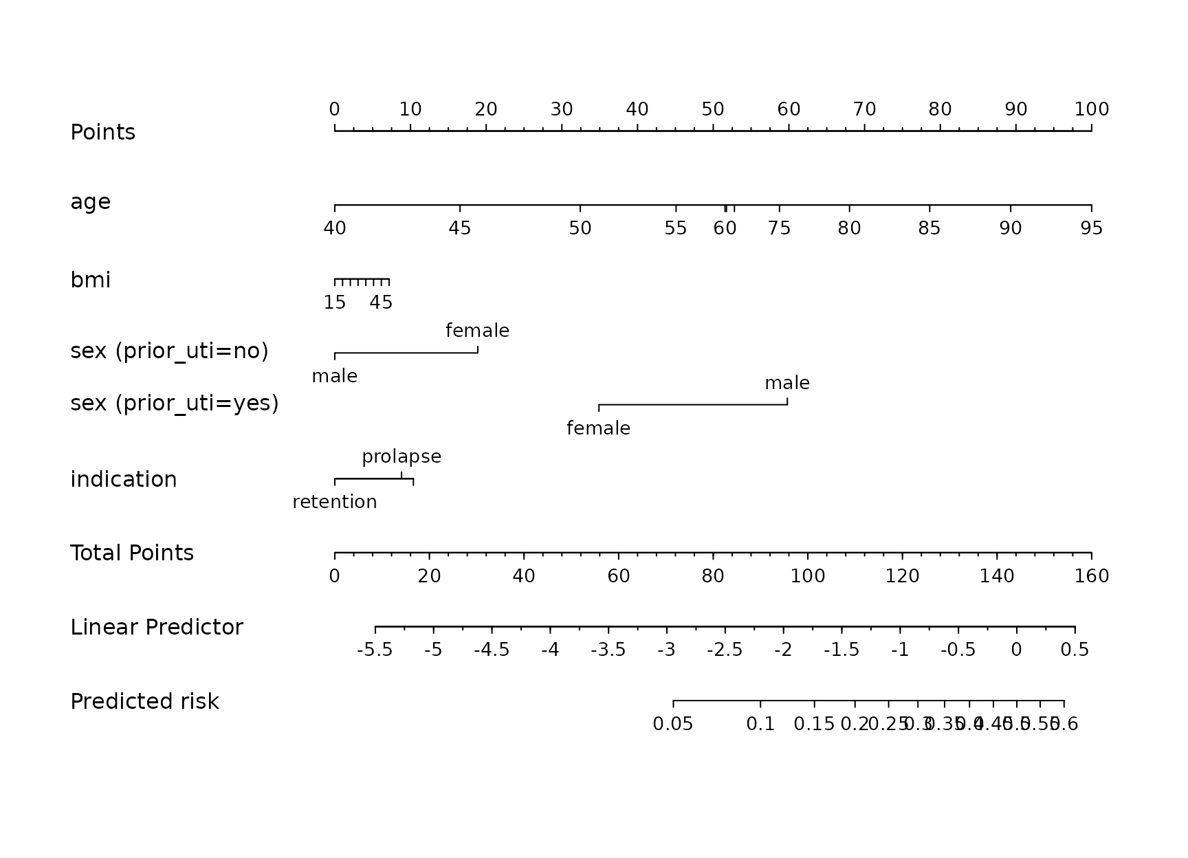
Passing out_dir writes the PDF, and the SVG and PNG when
svglite and ragg are installed. The third
article reads this nomogram back by hand.
What is not here yet
Imputation inside resampling, the flexible calibration curve,
selection, collinearity reporting and the Quarto manuscript. The roadmap
in the README says which version each belongs to. The pipeline above is
honest about its own limits in the place it would be easiest to hide
them, which is the note column of the validation table.