Reading the nomogram back • mysterymodel

library(mysterymodel)

A nomogram is a published instrument. Someone will read risks off it for real patients, by hand, years after the code that drew it stopped running. So the question mm_nomogram() answers is not “did rms draw something” but “does what it drew give the same answer as the model it was drawn from”.

This article does by hand what mm_nomogram() does internally, because the check is only convincing if you can see it.

cohort <- mm_synthetic_cohort(n = 500, prevalence = 0.11, seed = 1978)

project <- mm_project("uds", "event",
                      c("age", "bmi", "sex", "prior_uti"),
                      positive_class = 1, cohort = cohort, seed = 1978)

model <- suppressWarnings(
  mm_model(project, cohort, nonlinear = "age",
           interactions = list(c("prior_uti", "sex"))))

nom <- mm_nomogram(model, out_dir = NULL)
nom
#> <mm_nomogram>
#>   axes            age, bmi, sex (prior_uti=no), sex (prior_uti=yes)
#>   profiles checked 21 at tabulated ticks
#>   worst gap vs mm_predict() 1.11e-16 (tolerance 1e-06)
#>   off printed scale 8 tick profile(s) fall beyond the drawn axis
#>   between-tick reading      0.016 in risk at most, anywhere off the ticks
#>                             age is the coarsest axis
#>   mutually exclusive: exactly one axis of each group below applies
#>     sex (prior_uti=no)  |  sex (prior_uti=yes)
#>       read on sex, chosen by prior_uti
#>   axes        4 drawn for 4 predictor(s). Scoring two axes of one group double-counts the
#>               patient, which no check here can see because it
#>               happens on the printed sheet

plot(nom$nomogram)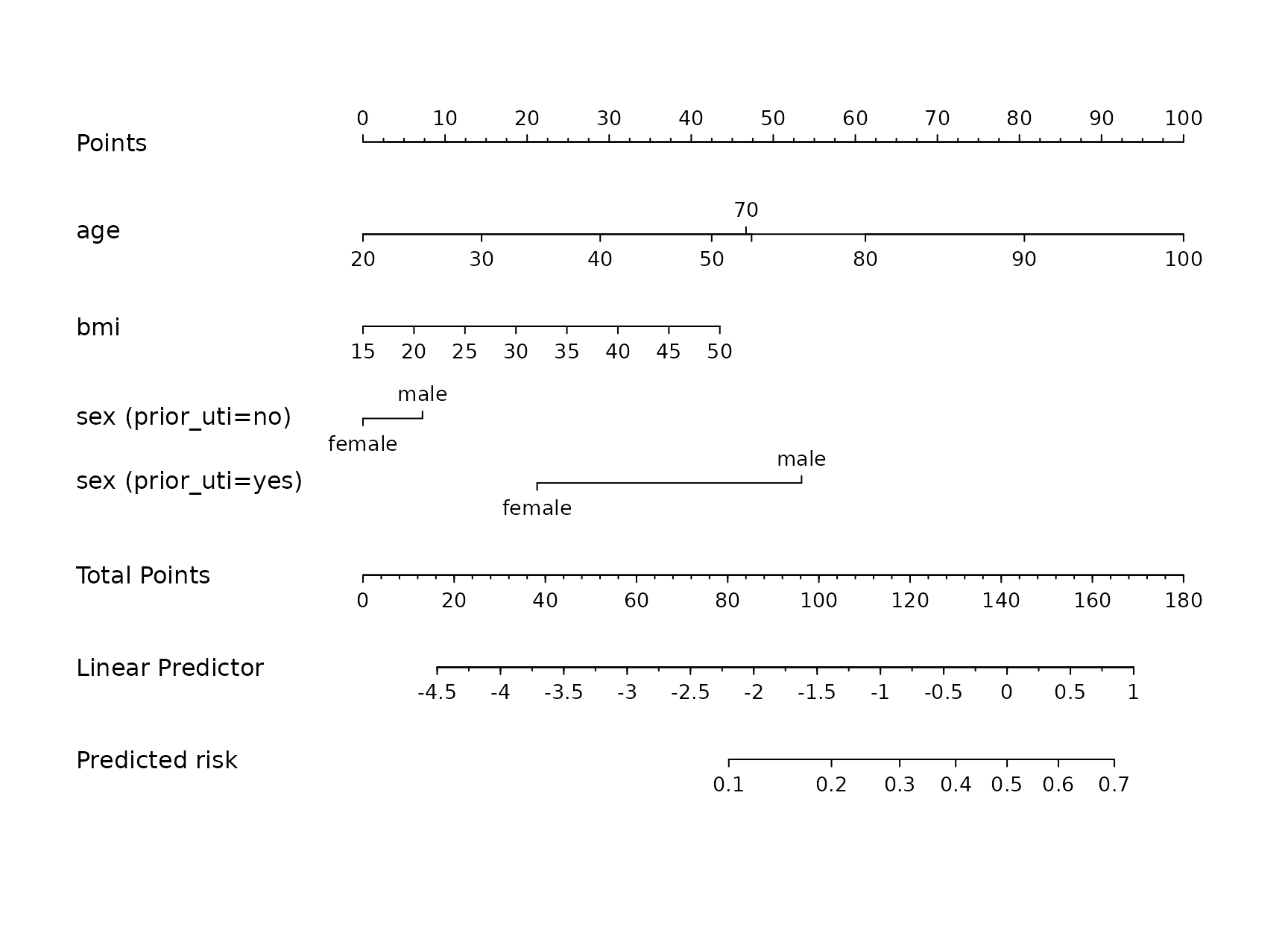

An interaction makes one variable appear on several axes

nom$axes
#> [1] "age"                 "bmi"                 "sex (prior_uti=no)" 
#> [4] "sex (prior_uti=yes)"

sex is not an axis. There are two axes that each hold both sex and prior_uti, and they are mutually exclusive: a patient with no prior UTI reads one, a patient with a prior UTI reads the other. A reader who gathered sex ticks from a single axis would get half the model.

mysterymodel:::mm_axis_values(nom$nomogram, project$predictors)
#> $age
#> [1]  20  30  40  50  60  70  80  90 100
#> 
#> $bmi
#> [1] 15 20 25 30 35 40 45 50
#> 
#> $sex
#> [1] "female" "male"  
#> 
#> $prior_uti
#> [1] "no"  "yes"

That is why the points reader gathers a predictor’s tabulated values across axes rather than off one, and why an axis contributes only when the profile matches every categorical value the axis holds fixed. Exactly one of the two applies to any patient, so nothing is counted twice and nothing is missed.

Reading one patient, by hand

Take a 70 year old woman with a BMI of 31 and a prior UTI.

patient <- data.frame(
  age       = 70,
  bmi       = 31,
  sex       = factor("female", levels = model$schema$predictors$sex$levels),
  prior_uti = factor("yes", levels = model$schema$predictors$prior_uti$levels)
)

Sum the points from every axis that applies:

total <- unname(mysterymodel:::mm_nomogram_points(nom$nomogram, patient))
total
#> [1] 87.7797

Convert the total to the linear predictor using the printed scale, then to a risk:

lp <- mysterymodel:::mm_total_to_lp(nom$nomogram, total)
c(total_points = total, linear_predictor = lp, risk = plogis(lp))
#>     total_points linear_predictor             risk 
#>       87.7797045       -1.9257965        0.1272166

unname(mysterymodel:::mm_nomogram_risk(nom$nomogram, patient))
#> [1] 0.1272166

Now ask the model the same question:

mm_predict(model, patient)$.pred
#> [1] 0.1272166

Neither calculation consulted the other. The reader above touched only nom$nomogram, a list of printed axis values; mm_predict() touched only the fitted lrm object. That independence is what makes the agreement evidence rather than a restatement.

abs(unname(mysterymodel:::mm_nomogram_risk(nom$nomogram, patient)) -
    mm_predict(model, patient)$.pred)
#> [1] 5.551115e-17

Every tick, not one patient

mm_nomogram() does not check a profile someone chose. It varies each predictor over all of its tabulated ticks while the others sit at their first, so every tick of every axis is exercised without taking the product of them all:

profiles <- mysterymodel:::mm_tick_profiles(nom$nomogram, model)
nrow(profiles)
#> [1] 21
head(profiles)
#>   age bmi    sex prior_uti
#> 1  20  15 female        no
#> 2  30  15 female        no
#> 3  40  15 female        no
#> 4  50  15 female        no
#> 5  60  15 female        no
#> 6  70  15 female        no

Those profiles come back again in the next section, where one of them turns out to be the reason the points-to-risk step is written the way it is.

read <- vapply(seq_len(nrow(profiles)), function(i)
  mysterymodel:::mm_nomogram_risk(nom$nomogram, profiles[i, , drop = FALSE]),
  numeric(1))
fitted <- mm_predict(model, profiles)$.pred

summary(abs(read - fitted))
#>      Min.   1st Qu.    Median      Mean   3rd Qu.      Max. 
#> 0.000e+00 0.000e+00 8.674e-18 1.355e-17 1.388e-17 1.110e-16
nom$worst_disagreement
#> [1] 1.110223e-16

Machine precision, across a model with a spline and an interaction. If the worst gap exceeded tolerance, mm_nomogram() would refuse to return at all:

mm_nomogram(model, out_dir = NULL, tolerance = 1e-20)
#> Error:
#> ! the nomogram disagrees with mm_predict() by 1.11e-16 at a tabulated profile, over the tolerance of 1e-20. A nomogram that does not reproduce its own model must not be published.

That refusal is the whole design. An instrument that does not reproduce its own model must not reach a manuscript, and the only moment anyone is in a position to notice is the moment it is drawn.

Why the points-to-risk step is a line and not an interpolation

The printed linear predictor axis is affine in total points, so the line through it is the exact mapping:

head(data.frame(points = nom$nomogram$lp$x,
                lp     = nom$nomogram$lp$x.real))
#>     points   lp
#> 1 16.26725 -4.5
#> 2 30.15746 -4.0
#> 3 44.04767 -3.5
#> 4 57.93788 -3.0
#> 5 71.82809 -2.5
#> 6 85.71830 -2.0

Interpolating between those ticks with clamped ends looks equivalent, and inside the printed range it is. The axis does not start at zero points, though, and nothing stops a patient from scoring below where it starts. Here is the lowest-scoring profile this model admits, a 20 year old woman at the bottom of the BMI range with no prior UTI:

totals <- vapply(seq_len(nrow(profiles)), function(i)
  unname(mysterymodel:::mm_nomogram_points(nom$nomogram,
                                           profiles[i, , drop = FALSE])),
  numeric(1))

lowest <- profiles[which.min(totals), , drop = FALSE]
lowest
#>   age bmi    sex prior_uti
#> 1  20  15 female        no
min(totals)
#> [1] 0
min(nom$nomogram$lp$x)
#> [1] 16.26725

Zero points, and the printed risk axis begins at 16.3. Clamped interpolation has nowhere to go, so it returns the value at the lowest printed tick:

clamped <- approx(nom$nomogram$lp$x, nom$nomogram$lp$x.real,
                  xout = min(totals), rule = 2)$y
exact <- mysterymodel:::mm_total_to_lp(nom$nomogram, min(totals))

c(clamped_risk = plogis(clamped),
  exact_risk   = plogis(exact),
  model_risk   = mm_predict(model, lowest)$.pred)
#> clamped_risk   exact_risk   model_risk 
#>  0.010986943  0.006147365  0.006147365

A risk of 1.1% reported for a patient whose risk is 0.6%, with no warning and nothing on the page to suggest the reading was out of range. That is the error this package shipped in its own first nomogram reader, and it is why mm_total_to_lp() uses the exact affine line instead and checks its linearity rather than trusting it: the function errors if the axis deviates from affine by more than 1e-8.

Reading between ticks has a cost, and here it is

Everything above holds at the nomogram’s own tabulated values. A clinician reads between them, and a spline curves between printed ticks where linear interpolation across them does not.

nom$reading_error
#> [1] 0.01603211

That is a bound: no reading taken anywhere between the printed ticks can differ from mm_predict() by more than that. It is a property of every printed nomogram and of every clinician reading one, not a defect of this package, and reporting its size is the alternative to leaving it unexamined.

The bound needs no search over combinations of predictors, because the error decomposes. Total points are additive and the printed risk axis is affine in them, so the discrepancy is the points-to-lp slope times the sum of each axis’s own interpolation error, and each of those is zero at that axis’s ticks. So the extremes of the sum are the sums of the extremes, one scan per axis finds them, and the worst total goes through the steepest part of the logistic curve:

nom$reading_error_by_axis
#>              lo           hi
#> age -0.06413393 5.356972e-02
#> bmi  0.00000000 8.881784e-16
c(lp_bound = nom$reading_error_lp,
  risk_bound = nom$reading_error,
  by_hand = unname(stats::plogis(nom$reading_error_lp / 2) -
                     stats::plogis(-nom$reading_error_lp / 2)))
#>   lp_bound risk_bound    by_hand 
#> 0.06413393 0.01603211 0.01603211

reading_error_by_axis is where to look when the bound is too large for comfort: it names the axis that needs more ticks. Fitting the same model without the spline makes the whole thing vanish, because linear terms make the printed points affine in the predictor and the interpolation exact:

linear <- suppressWarnings(
  mm_model(project, cohort, interactions = list(c("prior_uti", "sex"))))
mm_nomogram(linear, out_dir = NULL)$reading_error
#> [1] 4.440892e-16

The claim is worth testing rather than taking on the arithmetic above. Three hundred profiles drawn anywhere inside the printed axes, which is where a clinician reads, and the worst gap any of them produces:

ticks <- mysterymodel:::mm_axis_values(nom$nomogram, project$predictors)
set.seed(8)
anywhere <- data.frame(
  age = runif(300, min(ticks$age), max(ticks$age)),
  bmi = runif(300, min(ticks$bmi), max(ticks$bmi)),
  sex = factor(sample(model$schema$predictors$sex$levels, 300, TRUE),
               levels = model$schema$predictors$sex$levels),
  prior_uti = factor(sample(model$schema$predictors$prior_uti$levels, 300,
                            TRUE),
                     levels = model$schema$predictors$prior_uti$levels))
read_anywhere <- vapply(seq_len(nrow(anywhere)), function(i) unname(
  mysterymodel:::mm_nomogram_risk(nom$nomogram,
                                  anywhere[i, , drop = FALSE])), numeric(1))
c(worst_of_300 = max(abs(read_anywhere -
                           mm_predict(model, anywhere)$.pred)),
  bound = nom$reading_error)
#> worst_of_300        bound 
#>   0.01328614   0.01603211

Readings that fall off the drawn scale

nom$off_axis
#> [1] 8
range(nom$nomogram$lp$x)
#> [1]  16.26725 169.05955

A total outside the printed range is a reading a clinician cannot take, however well the arithmetic behind it works. Those profiles are counted rather than quietly reported as the nearest printed tick.

mysterymodel:::mm_off_axis(nom$nomogram, c(min(totals), total, 500))
#> [1]  TRUE FALSE  TRUE

Exporting

out <- file.path(tempdir(), "nomogram-article")
drawn <- mm_nomogram(model, out_dir = out, width = 13, height = 9)
#> wrote 3 nomogram file(s): /tmp/RtmpoBapOs/nomogram-article/uds_nomogram.pdf, /tmp/RtmpoBapOs/nomogram-article/uds_nomogram.svg, /tmp/RtmpoBapOs/nomogram-article/uds_nomogram.png
basename(drawn$files)
#> [1] "uds_nomogram.pdf" "uds_nomogram.svg" "uds_nomogram.png"

The landscape shape is the default because that is what the specification asks for. The PDF is always written; the SVG and PNG follow when svglite and ragg are installed, which is why they are suggested rather than required dependencies.

identical(drawn$fingerprint, model$fingerprint)
#> [1] TRUE

The fingerprint is the fit’s, so a figure in a manuscript can be tied to the coefficients that produced it. A nomogram whose fingerprint does not match the model table beside it was drawn from a different fit.