A complicated worked example

library(mysterymodel)

The other three articles each take one idea and follow it. This one does the opposite: it runs a whole study, on a cohort built to be awkward in every way the package has an opinion about, and compares four competing specifications against each other the way a supplement would. Every function in the package appears at least once, and the last section proves it rather than claiming it.

Read it as a worked example, not as a tutorial. If you want the pipeline in order, start with From a raw export to a checked nomogram.

1. An export built to be awkward

raw <- mm_synthetic_cohort(n = 900, prevalence = 0.12, years = 2018:2024,
                           repeat_frac = 0.12, seed = 1978)

set.seed(20261030)
n <- nrow(raw)

# Missingness, in two variables, overlapping on purpose.
raw$bmi[sample(n, 48)] <- NA
raw$indication[sample(n, 22)] <- NA

# A column that is the outcome under another name, which is the one mistake
# that makes its own output look better.
raw$triage_flag <- raw$event

# A marker that separates the classes completely without being a copy.
raw$marker <- ifelse(raw$event == 1L, runif(n, 8, 14), runif(n, 0, 6))

# A category that appears only after the temporal split.
raw$indication <- as.character(raw$indication)
late <- which(raw$year >= 2023)
raw$indication[sample(late, 14)] <- "urgency"
raw$indication <- factor(raw$indication)

# Rows no protocol would admit, and a handful with no patient identifier.
raw$age[sample(n, 30)] <- runif(30, 19, 38)
raw$bmi[sample(n, 12)] <- runif(12, 61, 74)
raw$pid[sample(n, 5)] <- NA

str(raw, give.attr = FALSE, vec.len = 2)
#> 'data.frame':    900 obs. of  10 variables:
#>  $ age        : num  48.7 67.1 54.7 94 73.2 ...
#>  $ bmi        : num  44.5 23.7 25.6 NA 31 ...
#>  $ sex        : Factor w/ 2 levels "female","male": 1 1 1 2 1 ...
#>  $ prior_uti  : Factor w/ 2 levels "no","yes": 1 1 2 2 1 ...
#>  $ indication : Factor w/ 4 levels "incontinence",..: 2 2 1 2 3 ...
#>  $ year       : int  2019 2021 2024 2020 2023 ...
#>  $ pid        : chr  "p0652" "p0462" ...
#>  $ event      : int  0 0 0 1 0 ...
#>  $ triage_flag: int  0 0 0 1 0 ...
#>  $ marker     : num  4.8 4.63 ...

The truth behind the generated part is known, which is what makes a specification comparison meaningful at all:

attr(raw, "truth")$formula
#> [1] "event ~ 0.0011*(age-62)^2 + 0.045*(bmi-29) + 0.35*male + 0.80*prior_uti + 0.60*prior_uti:male"
round(attr(raw, "truth")$coefficients, 4)
#>     intercept        age_sq           bmi      sex_male prior_uti_yes   uti_by_male 
#>       -2.7343        0.0011        0.0450        0.3500        0.8000        0.6000

2. What is in the export, before any decision

described <- mm_eda(raw, by = "event",
                    vars = c("age", "bmi", "sex", "prior_uti",
                             "indication", "marker"))
described
#> <mm_eda>  900 rows, by event
#>       variable           statistic           Overall         event = 0
#>  (denominator)                   n               900               798
#>            age           mean (SD)       61.4 (13.6)       61.2 (13.2)
#>            age   median (p25, p75) 62.2 (52.7, 70.3) 62.0 (52.7, 70.0)
#>            age      missing, n (%)          0 (0.0%)          0 (0.0%)
#>            bmi           mean (SD)        29.4 (7.4)        29.2 (7.3)
#>            bmi   median (p25, p75) 29.2 (25.0, 33.1) 29.0 (24.9, 33.0)
#>            bmi      missing, n (%)         47 (5.2%)         41 (5.1%)
#>            sex       female, n (%)       657 (73.0%)       598 (74.9%)
#>            sex         male, n (%)       243 (27.0%)       200 (25.1%)
#>            sex      missing, n (%)          0 (0.0%)          0 (0.0%)
#>      prior_uti           no, n (%)       595 (66.1%)       544 (68.2%)
#>      prior_uti          yes, n (%)       305 (33.9%)       254 (31.8%)
#>      prior_uti      missing, n (%)          0 (0.0%)          0 (0.0%)
#>     indication incontinence, n (%)       448 (50.9%)       392 (50.3%)
#>     indication     prolapse, n (%)       177 (20.1%)       158 (20.3%)
#>     indication    retention, n (%)       241 (27.4%)       217 (27.8%)
#>     indication      urgency, n (%)         14 (1.6%)         13 (1.7%)
#>     indication      missing, n (%)         20 (2.2%)         18 (2.3%)
#>         marker           mean (SD)         3.8 (3.0)         3.0 (1.7)
#>         marker   median (p25, p75)    3.3 (1.7, 5.0)    3.0 (1.5, 4.5)
#>         marker      missing, n (%)          0 (0.0%)          0 (0.0%)
#>          event = 1
#>                102
#>        63.1 (16.6)
#>  63.7 (50.3, 75.9)
#>           0 (0.0%)
#>         31.0 (8.2)
#>  30.4 (25.4, 34.9)
#>           6 (5.9%)
#>         59 (57.8%)
#>         43 (42.2%)
#>           0 (0.0%)
#>         51 (50.0%)
#>         51 (50.0%)
#>           0 (0.0%)
#>         56 (56.0%)
#>         19 (19.0%)
#>         24 (24.0%)
#>           1 (1.0%)
#>           2 (2.0%)
#>         10.6 (1.7)
#>   10.4 (9.2, 11.8)
#>           0 (0.0%)
#> 
#> missing: bmi 5.2%, indication 2.2%

That print method is print.mm_eda. The object underneath carries the table, the missingness ordered worst first, and the duplicate count:

described$missing
#>     variable n_missing pct_missing
#> 2        bmi        47         5.2
#> 5 indication        20         2.2
#> 1        age         0         0.0
#> 3        sex         0         0.0
#> 4  prior_uti         0         0.0
#> 6     marker         0         0.0
c(rows = described$n, duplicated_rows = described$duplicates,
  stratified_by = described$by)
#>            rows duplicated_rows   stratified_by 
#>           "900"             "0"         "event"

Every cell in that table is built by one of four formatters, so a table cannot be internally inconsistent about how it rounds:

c(count       = mysterymodel:::mm_count(nrow(raw)),
  n_pct       = mysterymodel:::mm_n_pct(sum(raw$event), nrow(raw)),
  mean_sd     = mysterymodel:::mm_mean_sd(raw$age, digits = 1),
  median_iqr  = mysterymodel:::mm_median_iqr(raw$marker, digits = 2))
#>               count               n_pct             mean_sd          median_iqr 
#>               "900"       "102 (11.3%)"       "61.4 (13.6)" "3.28 (1.70, 5.02)"

3. Eligibility, with a ledger that reconciles

Five rules. One of them cannot be evaluated for rows with no BMI, so those rows leave under their own heading rather than passing.

eligible <- mm_clean(raw, rules = list(
  "aged 40 or over"      = ~ age >= 40,
  "plausible BMI"        = ~ bmi >= 16 & bmi <= 60,
  "indication recorded"  = ~ !is.na(indication),
  "patient identified"   = ~ !is.na(pid),
  "indication in scope"  = ~ indication != "urgency"
), label = "urodynamics studies as exported")

eligible
#> <mm_cohort>  900 in, 741 out, 159 excluded
#>      900  urodynamics studies as exported
#>      -54  aged 40 or over (did not meet the criterion)
#>      846  remaining
#>      -24  plausible BMI (did not meet the criterion)
#>      822  remaining
#>      -45  plausible BMI (criterion could not be determined for these rows)
#>      777  remaining
#>      -19  indication recorded (did not meet the criterion)
#>      758  remaining
#>       -5  patient identified (did not meet the criterion)
#>      753  remaining
#>      -12  indication in scope (did not meet the criterion)
#>      741  remaining

eligible$ledger[, c("step", "rule", "n_excluded", "n_after", "reason")]
#>   step                            rule n_excluded n_after
#> 1    0 urodynamics studies as exported         NA     900
#> 2    1                 aged 40 or over         54     846
#> 3    2                   plausible BMI         24     822
#> 4    2                   plausible BMI         45     777
#> 5    3             indication recorded         19     758
#> 6    4              patient identified          5     753
#> 7    5             indication in scope         12     741
#>                                             reason
#> 1                                  starting cohort
#> 2                       did not meet the criterion
#> 3                       did not meet the criterion
#> 4 criterion could not be determined for these rows
#> 5                       did not meet the criterion
#> 6                       did not meet the criterion
#> 7                       did not meet the criterion
with(eligible, c(in_ = n_in, out = n_out, excluded = n_excluded,
                 reconciles = n_in - n_excluded == n_out))
#>        in_        out   excluded reconciles 
#>        900        741        159          1

Dropping urgency here is a decision, not a technicality. Left in, it would reach the held-out rows and mm_predict() would refuse to score them, because the development rows never saw that level. Making it an eligibility rule puts the exclusion in the flow diagram where a reader can argue with it.

cohort <- eligible$data
nrow(cohort)
#> [1] 741

4. Four plans, written down before anything is fitted

Four specifications, differing one step at a time, so that each contrast is attributable to one decision.

predictors <- c("age", "bmi", "sex", "prior_uti", "indication")

plan <- list(
  A = mm_project("uds-a", "event", predictors, positive_class = 1,
                 cohort = cohort, seed = 1978),
  B = mm_project("uds-b", "event", predictors, positive_class = 1,
                 cohort = cohort, seed = 1978),
  C = mm_project("uds-c", "event", predictors, positive_class = 1,
                 cohort = cohort, cluster_id = "pid", seed = 1978),
  D = mm_project("uds-d", "event", predictors, positive_class = 1,
                 cohort = cohort, split_var = "year", split_at = 2023,
                 cluster_id = "pid", seed = 1978))

plan$D
#> <mm_project: uds-d>
#>   outcome    event (event = 1)
#>   predictors 5: age, bmi, sex, prior_uti, indication
#>   split      year < 2023 develops, the rest is held out
#>   cluster    pid
#>   shape      every continuous predictor linear
#>   seed       1978

analysis	shape	split	resampling unit
A	additive	none	row
B	spline on age	none	row
C	spline, plus prior_uti by sex	none	whole patient
D	as C	develop before 2023	whole patient

5. The leakage scan, before any of them is fitted

The two planted problems are different findings and the package treats them differently. Taking the development frame of plan D by hand:

parts <- mysterymodel:::mm_split(plan$D, cohort)
c(development = nrow(parts$dev), held_out = nrow(parts$held))
#> development    held_out 
#>         551         190

y_dev <- mysterymodel:::mm_event_indicator(parts$dev$event, 1)
c(events = sum(y_dev), prevalence = round(mean(y_dev), 4))
#>     events prevalence 
#>    64.0000     0.1162

probe <- mm_project("probe", "event",
                    c(predictors, "triage_flag", "marker"),
                    positive_class = 1, seed = 1978)
found <- mysterymodel:::mm_leakage(probe, parts$dev, y = y_dev)

do.call(rbind, lapply(found, function(f) data.frame(
  tier = f$tier, predictor = f$predictor, kind = f$kind,
  n_compared = f$n_compared, n_missing = f$n_missing)))
#>   tier   predictor       kind n_compared n_missing
#> 1    1 triage_flag       copy        551         0
#> 2    3      marker separation        551         0

for (f in found) cat(sprintf("tier %d, %s:\n", f$tier, f$predictor),
                     strwrap(f$detail, 76, prefix = "  "), sep = "\n")
#> tier 1, triage_flag:
#> 
#>   reads as binary with 1 is the event, and reproduces the outcome on every
#>   one of the 551 compared row(s)
#> tier 3, marker:
#> 
#>   every event lies above every non-event: non-events reach 5.995189, events
#>   start at 8.147008

Raising those findings blocks on the first and warns on the second:

blocked <- tryCatch(
  mysterymodel:::mm_report_leakage(found, "event"),
  error = function(e) conditionMessage(e))
cat(strwrap(blocked, 78), sep = "\n")
#> outcome leakage: predictor `triage_flag` reads as binary with 1 is the event,
#> and reproduces the outcome on every one of the 551 compared row(s). A
#> predictor carrying `event` is not predicting it, and a model given one
#> reports near-perfect discrimination, which reads as success. Remove it before
#> fitting.

The detection reads values, never names. A column becomes a candidate copy only where reading it as 0/1 involves no guessing:

str(mysterymodel:::mm_binary_forms(cohort$triage_flag))
#> List of 1
#>  $ :List of 2
#>   ..$ code : int [1:741] 0 0 0 0 0 0 0 0 0 0 ...
#>   ..$ label: chr "1 is the event"
length(mysterymodel:::mm_binary_forms(cohort$indication))
#> [1] 0
length(mysterymodel:::mm_binary_forms(cohort$marker))
#> [1] 0

Neither triage_flag nor marker is in the four plans, which is why they fit at all. Asking for the leaked one is refused:

mm_model(probe, cohort)
#> Error:
#> ! outcome leakage: predictor `triage_flag` reads as binary with 1 is the event, and reproduces the outcome on every one of the 741 compared row(s). A predictor carrying `event` is not predicting it, and a model given one reports near-perfect discrimination, which reads as success. Remove it before fitting.

6. The eligibility arithmetic, by hand

The rule that decides which rows are modelled is the same one validation reads, and it is available on its own:

dev_eligible <- mysterymodel:::mm_evaluable(plan$D, parts$dev,
                                            require_cluster = TRUE)
held_eligible <- mysterymodel:::mm_evaluable(plan$D, parts$held,
                                             require_cluster = FALSE)

rbind(development = unlist(dev_eligible[c("n_total", "n_scored", "n_excluded",
                                          "missing_predictor",
                                          "missing_outcome", "missing_both")]),
      held_out = unlist(held_eligible[c("n_total", "n_scored", "n_excluded",
                                        "missing_predictor",
                                        "missing_outcome", "missing_both")]))
#>             n_total n_scored n_excluded missing_predictor missing_outcome
#> development     551      551          0                 0               0
#> held_out        190      190          0                 0               0
#>             missing_both
#> development            0
#> held_out               0

Nothing is excluded here, because section 3 made completeness an eligibility rule. On a cohort where something was, the sentence that reaches the note column reads like this:

pretend <- parts$held
pretend$bmi[1:7] <- NA
pretend$event[8:11] <- NA
cat(strwrap(mysterymodel:::mm_eligibility_note(
  mysterymodel:::mm_evaluable(plan$D, pretend)), 76), sep = "\n")
#> 179 of 190 row(s) scored, 11 excluded (7 for a missing predictor, 4 for a
#> missing outcome; bmi 7, event 4). Complete case, so these estimates assume
#> the exclusions are uninformative, which is an assumption and not a finding

A fingerprint of the rows themselves, which is how validation later refuses a cohort that is not the one a model was fitted on:

substr(mysterymodel:::mm_sample_digest(plan$D, parts$dev), 1, 24)
#> [1] "a97f8dd9ff7e7f0be8654991"

7. Fitting all four

shape <- list(
  A = list(nonlinear = NULL,  interactions = NULL),
  B = list(nonlinear = "age", interactions = NULL),
  C = list(nonlinear = "age", interactions = list(c("prior_uti", "sex"))),
  D = list(nonlinear = "age", interactions = list(c("prior_uti", "sex"))))

fits <- lapply(names(plan), function(k) suppressWarnings(
  mm_model(plan[[k]], cohort, nonlinear = shape[[k]]$nonlinear,
           interactions = shape[[k]]$interactions, knots = 4)))
names(fits) <- names(plan)

fits$D
#> <mm_model: uds-d>
#>   formula    .mm_y ~ rms::rcs(age, 4) + bmi + sex + prior_uti + indication +     prior_uti:sex
#>   developed  551 rows, 64 events
#>   held out   190 rows
#>   parameters 9 non-intercept, 710 short of the sample they need
#>   apparent C 0.7116
#>   fingerprint 3b00d7880d0bada1

do.call(rbind, lapply(names(fits), function(k) {
  m <- fits[[k]]
  data.frame(analysis = k, n_supplied = m$n_supplied, n_dev = m$n_dev,
             events = m$events_dev, n_held = m$n_held,
             parameters = m$adequacy$parameters,
             apparent_C = round(unname(m$fit$stats["C"]), 4),
             fingerprint = substr(m$fingerprint, 1, 10))
}))
#>   analysis n_supplied n_dev events n_held parameters apparent_C fingerprint
#> 1        A        741   741     83      0          6     0.6425  20486eeb8c
#> 2        B        741   741     83      0          8     0.6584  b40edbe891
#> 3        C        741   741     83      0          9     0.6695  93ca893c56
#> 4        D        551   551     64    190          9     0.7116  3b00d7880d

The sample-size gate is reported per analysis, and it is the honest answer for a cohort this size once the parameter count rises:

fits$C$adequacy
#> <mm_adequacy>  adequate: FALSE
#>   development 741 rows, 83 events (11.2%)
#>   parameters  9 non-intercept, 9.2 events each (description, not the criterion)
#>   shrinkage   0.739 expected, heuristic
#>   requires    1716 rows, 193 events (Riley, from the fitted R2 of 0.090)
#>   741 rows is 975 short of the 1716 a model of 9 parameter(s) needs at 11.2% prevalence for 90% shrinkage

That gate can also be asked a counterfactual question, which is the one it cannot answer from the fit alone: what would this model have needed if its explanatory performance were the 0.25 a previous study reported?

mysterymodel:::mm_adequacy(
  n = fits$C$n_dev, events = fits$C$events_dev,
  parameters = fits$C$adequacy$parameters, nagelkerke = 0.25,
  likelihood_ratio = unname(fits$C$fit$stats[["Model L.R."]]))
#> <mm_adequacy>  adequate: TRUE
#>   development 741 rows, 83 events (11.2%)
#>   parameters  9 non-intercept, 9.2 events each (description, not the criterion)
#>   shrinkage   0.739 expected, heuristic
#>   requires    597 rows, 67 events (Riley, from the fitted R2 of 0.250)
#>   741 rows meets the 597 a model of 9 parameter(s) needs

What a deployed prediction is allowed to receive, recorded at fit time and reconstructible on demand:

schema <- mysterymodel:::mm_schema(plan$D, parts$dev)
str(schema$predictors[c("age", "indication")])
#> List of 2
#>  $ age       :List of 2
#>   ..$ type : chr "numeric"
#>   ..$ range: num [1:2] 40.2 95
#>  $ indication:List of 2
#>   ..$ type  : chr "categorical"
#>   ..$ levels: chr [1:3] "incontinence" "prolapse" "retention"
identical(schema$predictors, fits$D$schema$predictors)
#> [1] TRUE

The shape plan B buys, and what it costs

A and B differ in one declared decision: B gives age a restricted cubic spline. Both allocations were written down in section 4, so what follows is not a choice being made now; it is what the choice already made amounts to. mm_splines() fits each continuous predictor both ways and reports the difference, which is the arithmetic the contrast table below needs in order to mean anything.

shapes <- mm_splines(plan$B, cohort, knots = 4)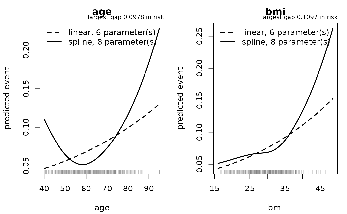

shapes$summary[, c("predictor", "parameters_linear", "parameters_spline",
                   "largest_risk_gap", "at_value")]
#>   predictor parameters_linear parameters_spline largest_risk_gap at_value
#> 1       age                 6                 8       0.09783402     95.0
#> 2       bmi                 6                 8       0.10965151     48.6

Two continuous predictors and the same two extra parameters each. The generating model behind this cohort carries a quadratic age term and a linear bmi term:

attr(raw, "truth")$formula
#> [1] "event ~ 0.0011*(age-62)^2 + 0.045*(bmi-29) + 0.35*male + 0.80*prior_uti + 0.60*prior_uti:male"

The age gap is the larger of the two, which is the ordering the truth predicts. It is worth being careful about how much that ordering proves, because bmi is linear by construction and its gap is not small either, and both maxima sit at the very top of their observed ranges. A spline is least constrained where the data runs out, so largest_risk_gap is partly a statement about curvature and partly a statement about where this cohort stops. Reading it without the rug below would attribute all of it to the first.

The curves are adjusted: every other predictor sits at the reference profile, which is returned because an adjusted curve means nothing without the values it was adjusted to.

shapes$reference
#>    age  bmi    sex prior_uti   indication
#> 1 63.5 29.1 female        no incontinence

Standing somewhere else moves them. Here is the same comparison for a patient at the other end of both categorical axes, which is a different question and has a different answer:

elsewhere <- mm_splines(plan$B, cohort, predictors = "age",
                        at = list(sex = "male", prior_uti = "yes",
                                  indication = "retention"),
                        plot = FALSE)
rbind(reference = shapes$summary[shapes$summary$predictor == "age",
                                 c("largest_risk_gap", "at_value")],
      elsewhere = elsewhere$summary[, c("largest_risk_gap", "at_value")])
#>           largest_risk_gap at_value
#> reference       0.09783402       95
#> elsewhere       0.15569960       95

invisible(mm_splines(plan$B, cohort, knots = 4))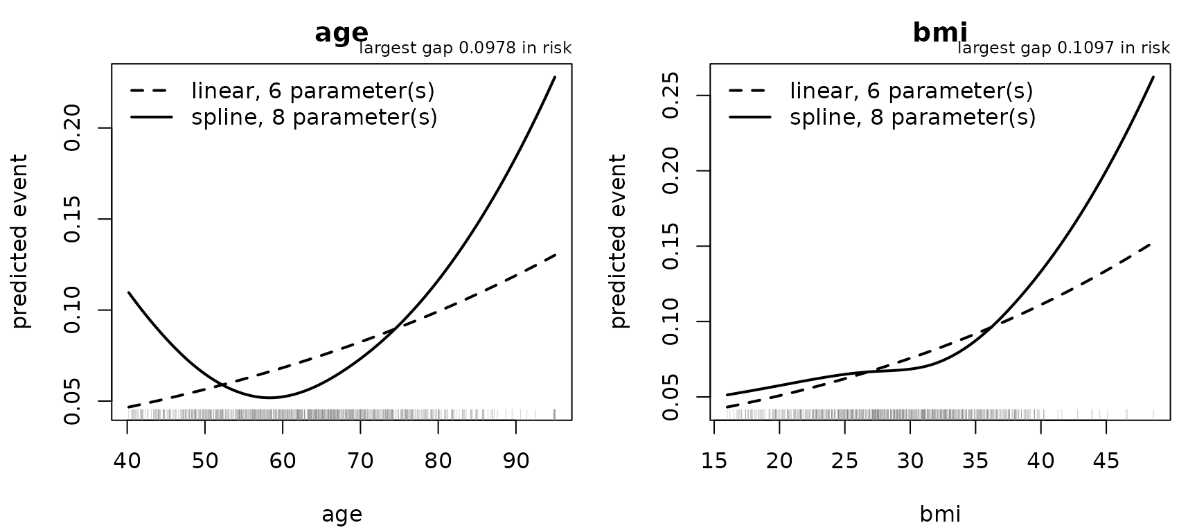

The dashed line is A’s allocation and the solid line is B’s. The rug is where the data actually is, and it is the part of the picture that explains the table above: both maxima are at the right-hand end of their panels, where the rug thins out and the spline has least holding it down. That is a real feature of the allocation rather than an artefact to be corrected, and it is the reason a clinician reading a nomogram built on plan B should be told which part of each axis the cohort actually covered.

What the figure does not carry is a binned observed event rate, however natural it would look underneath two fitted curves. A marginal event rate and an adjusted curve are different quantities, and an eye given both will compare them anyway.

Nor is there a p-value here, and that absence is deliberate. rms will give you one: the aggregate nonlinear term sits in the anova table immediately beside the interaction block.

old <- options(datadist = fits$B$datadist)
anova(fits$B$fit, test = "LR")[c("age", " Nonlinear"), ]
#>            Chi-Square d.f.          P
#> age         10.419639    3 0.01531606
#>  Nonlinear   6.275555    2 0.04337911
options(old)

Fitting the spline, reading that row, and dropping back to a straight line when it is not significant would make the model’s shape a function of the outcome. The optimism of that choice is corrected by nothing downstream, which is the same error as choosing an interaction on the development data and then validating the chosen model as though it had been prespecified. The allocation belonged in section 4, and that is where it was.

The cost side is the parameter budget, which the sample-size gate was already unhappy about:

data.frame(
  analysis = c("A", "B"),
  parameters = c(fits$A$adequacy$parameters, fits$B$adequacy$parameters),
  required_n = ceiling(c(fits$A$adequacy$required_n,
                         fits$B$adequacy$required_n)),
  short_by = ceiling(c(fits$A$adequacy$short_by,
                       fits$B$adequacy$short_by)),
  shrinkage = round(c(fits$A$adequacy$heuristic_shrinkage,
                      fits$B$adequacy$heuristic_shrinkage), 3))
#>   analysis parameters required_n short_by shrinkage
#> 1        A          6       1658      917     0.749
#> 2        B          8       1760     1019     0.735

So B buys a shape worth a tenth or two of predicted risk towards the top of the age range, where this cohort is thinnest, and pays for it with two parameters the sample is already short of. Both halves of that sentence are reported, and neither is a recommendation.

The block plans C and D declare

C and D add prior_uti by sex, prespecified in section 4 and planted in the generating model. mm_interactions() tests it as an addition to the main-effects model, and reports what the test rests on rather than only its p-value. A second candidate is included that nobody declared, to show that a screen of two blocks is reported as a screen of two blocks.

blocks <- mm_interactions(
  plan$C, cohort,
  candidates = list(c("prior_uti", "sex"), c("sex", "indication")),
  nonlinear = "age", adjustment = "holm")
#> mm_interactions(): 2 prespecified block(s), LR test, multiplicity holm
blocks
#> <mm_interaction_screen>  prespecified, LR test
#>   development 741 rows, 83 events, 8 parameter(s) before any block
#>   candidates  2 block(s) considered, 3 parameter(s) of candidate complexity in total
#>               a model taking every one of them would spend 11 parameter(s) on 83 event(s), 7.5 each
#>   prior_uti x sex        tested  chi2=4.353 df=1 p=0.0369 p.adj=0.0739
#>   sex x indication       tested  chi2=1.664 df=2 p=0.4351 p.adj=0.4351
#>   Evidence about blocks, not a model. Nothing here has been added to
#>   a model, and a small p-value is not a reason to add it: the
#>   optimism of choosing on these data is not corrected by this
#>   function.

blocks$screen[, c("interaction", "statistic", "degrees_freedom", "p_value",
                  "p_adjusted", "added_rank", "smallest_cell", "lr_agrees")]
#>        interaction statistic degrees_freedom    p_value p_adjusted added_rank
#> 1  prior_uti x sex  4.352836               1 0.03694738 0.07389476          1
#> 2 sex x indication  1.664190               2 0.43513667 0.43513667          2
#>   smallest_cell lr_agrees
#> 1            70      TRUE
#> 2            40      TRUE

added_rank is the dimension each block actually adds to the design matrix, and no test is reported unless it equals the columns the block contributes: that is what stops a block which adds nothing from coming back with a p-value near one, which would read as evidence of no interaction. lr_agrees records that the deviance difference and rms::anova(test = "LR") agreed, checked on this call rather than once in a test file.

The planted block is the one the plan declared. The other was included to be counted, and it is: the candidate budget is two blocks and three parameters whichever of them survives, which is the complexity the analysis spent even though plan C contains only one of them.

c(candidates = blocks$n_candidates,
  candidate_parameters = blocks$candidate_parameters,
  parameters_in_plan_C = fits$C$adequacy$parameters)
#>           candidates candidate_parameters parameters_in_plan_C 
#>                    2                    3                    9

Nothing above changed a model. Plan C contains the block because section 4 said so, not because this table did.

8. Validating all four

checked <- lapply(names(fits), function(k) suppressWarnings(
  mm_validate(fits[[k]], cohort, B = 60,
              full_process = k %in% c("C", "D"))))
names(checked) <- names(fits)

checked$D
#> <mm_validation>  full-process: TRUE
#>   columns: n, events/non-events, c-statistic with its 95% DeLong interval where one is estimable
#>   apparent                 n=551   64/487 C=0.7116 (0.6386-0.7846)
#>   bootstrap, fixed model   n=551   64/487 C=0.6647 no interval, see note  slope=0.8200
#>   bootstrap, full process  n=551   64/487 C=0.6752 no interval, see note  slope=0.8446
#>   held out                 n=190   19/171 C=0.4974 (0.3275-0.6673)  slope=0.2950
#>   Full process re-derives knot placement, datadist, factor levels per resample; 60 of 60 valid.
#>   Its correction carries a Monte Carlo standard error of 0.00429 on C; rms does not return
#>   the per-resample values its own row is averaged over, so the
#>   same figure cannot be given for the fixed-model row.

basis_c <- function(v, basis) {
  value <- v$metrics$c_stat[v$metrics$basis == basis]
  if (!length(value)) NA_real_ else round(value, 4)
}
do.call(rbind, lapply(names(checked), function(k) data.frame(
  analysis  = k,
  apparent  = basis_c(checked[[k]], "apparent"),
  fixed     = basis_c(checked[[k]], "bootstrap, fixed model"),
  process   = basis_c(checked[[k]], "bootstrap, full process"),
  held_out  = basis_c(checked[[k]], "held out"),
  unit      = if (is.null(checked[[k]]$fixed_model$clustered_by)) "row" else
    checked[[k]]$fixed_model$clustered_by)))
#>   analysis apparent  fixed process held_out unit
#> 1        A   0.6425 0.6056      NA       NA  row
#> 2        B   0.6584 0.6172      NA       NA  row
#> 3        C   0.6695 0.6234  0.6325       NA  pid
#> 4        D   0.7116 0.6647  0.6752   0.4974  pid

Analysis D is the one to read, and it is sobering. Apparent discrimination of 0.71 corrects to 0.66, and the rows the split reserved give this:

held_row <- checked$D$metrics[checked$D$metrics$basis == "held out", ]
c(n = held_row$n, events = held_row$events,
  C = round(held_row$c_stat, 4),
  lower = round(held_row$c_lower, 4), upper = round(held_row$c_upper, 4))
#>        n   events        C    lower    upper 
#> 190.0000  19.0000   0.4974   0.3275   0.6673

Twenty-odd events support an interval running from well below chance to well above it, so the point estimate is not evidence of anything much. That is what a held-out sample this size can tell you, and it is the number a reader will quote.

Contrasts, each attributable to one decision

corrected <- vapply(checked, basis_c, numeric(1),
                    basis = "bootstrap, fixed model")
data.frame(
  contrast = c("B less A", "C less B", "D less C"),
  decision = c("a spline on age", "an interaction, and clustered resampling",
               "a temporal split"),
  difference = round(c(corrected[["B"]] - corrected[["A"]],
                       corrected[["C"]] - corrected[["B"]],
                       corrected[["D"]] - corrected[["C"]]), 4))
#>   contrast                                 decision difference
#> 1 B less A                          a spline on age     0.0116
#> 2 C less B an interaction, and clustered resampling     0.0062
#> 3 D less C                         a temporal split     0.0413

Read those with the caution the validation article gives: the two bootstrap columns are different estimators, and D’s development sample is smaller than C’s because the split reserved rows, so “D less C” mixes two changes. A supplement would say so in the same sentence as the number.

The pieces a validation row is made of

p_held <- mm_predict(fits$D, parts$held)$.pred
y_held <- mysterymodel:::mm_event_indicator(parts$held$event, 1)
reference <- mean(y_dev) * (1 - mean(y_dev))

by_hand <- mysterymodel:::mm_metrics(p_held, y_held, basis = "held out",
                                     note = "assembled here",
                                     reference = reference)
by_hand[, c("basis", "n", "events", "c_stat", "c_lower", "c_upper",
            "cal_intercept", "cal_slope", "brier", "brier_ref",
            "brier_scaled")]
#>      basis   n events    c_stat   c_lower   c_upper cal_intercept cal_slope
#> 1 held out 190     19 0.4973838 0.3274533 0.6673143    -0.2831659 0.2949611
#>        brier brier_ref brier_scaled
#> 1 0.09344929 0.1026611   0.08972992

The apparent row is the one place those calibration terms are an identity rather than an estimate, and the function that withholds them can be shown doing both:

apparent <- mysterymodel:::mm_metrics(
  mm_predict(fits$D, parts$dev)$.pred, y_dev, basis = "apparent")
withheld <- mysterymodel:::mm_withhold_identity_calibration(apparent)

rbind(computed = c(intercept = apparent$cal_intercept,
                   slope = apparent$cal_slope),
      reported = c(withheld$cal_intercept, withheld$cal_slope))
#>             intercept slope
#> computed -1.40273e-15     1
#> reported           NA    NA

The full-process bootstrap, on its own

process <- suppressWarnings(
  mysterymodel:::mm_full_process(fits$D, cohort, B = 60, min_valid = 48))

c(valid = process$valid, of = process$B, adequate = process$adequate,
  reference = round(process$no_information_brier, 5))
#>     valid        of  adequate reference 
#>  60.00000  60.00000   1.00000   0.10266
process$covers
#> [1] "knot placement" "datadist"       "factor levels"
round(rbind(optimism = process$optimism, corrected = process$corrected), 5)
#>            c_stat cal_intercept cal_slope    brier brier_scaled
#> optimism  0.03635       0.04386    0.1554 -0.00121      0.01179
#> corrected 0.67524      -0.04386    0.8446  0.09578      0.06701

It refuses a frame that is not the one the model was fitted on, which is a check on the rows and not on their number:

altered <- parts$dev
altered$age <- rev(altered$age)
tryCatch(mysterymodel:::mm_same_development(fits$D, altered, "this contrast"),
         error = function(e) cat(strwrap(conditionMessage(e), 78), sep = "\n"))
#> `cohort` has the same number of evaluable development rows as the model was
#> fitted on, and they are not the same rows: the development fingerprint is
#> 3ee3aa7c8f36 and the model was fitted on a97f8dd9ff7e. this contrast would be
#> computed on data the model never saw. If only the row order changed, pass the
#> cohort in the order it was fitted in.

Resampling the patient rather than the row

dev_rows <- parts$dev
set.seed(4)
by_row     <- mysterymodel:::mm_resample(dev_rows, cluster_id = NULL)
by_patient <- mysterymodel:::mm_resample(dev_rows, cluster_id = "pid")

twins <- names(which(table(dev_rows$pid) == 2L))
rows_drawn <- table(factor(dev_rows$pid[by_patient], levels = twins))

c(rows = nrow(dev_rows),
  row_draw = length(by_row), patient_draw = length(by_patient),
  patients_with_two_visits = length(twins),
  all_even = all(rows_drawn %% 2L == 0L))
#>                     rows                 row_draw             patient_draw 
#>                      551                      551                      536 
#> patients_with_two_visits                 all_even 
#>                       40                        1

And a resample count is a count:

mysterymodel:::mm_check_resamples(60.0)
mysterymodel:::mm_check_resamples(2.7)
#> Error:
#> ! `B` is 2.7, which is not a whole number of resamples. Truncating it to 2 would answer a question that was not asked.

9. The nomogram, read back by hand

figures <- file.path(tempdir(), "worked-example")
nom <- mm_nomogram(fits$D, out_dir = figures, width = 13, height = 9)
#> wrote 3 nomogram file(s): /tmp/Rtmp1Zg5XE/worked-example/uds-d_nomogram.pdf, /tmp/Rtmp1Zg5XE/worked-example/uds-d_nomogram.svg, /tmp/Rtmp1Zg5XE/worked-example/uds-d_nomogram.png
nom
#> <mm_nomogram>
#>   axes            age, bmi, sex (prior_uti=no), sex (prior_uti=yes), indication
#>   profiles checked 27 at tabulated ticks
#>   worst gap vs mm_predict() 5.55e-17 (tolerance 1e-06)
#>   between-tick reading      0.00484 in risk at most, anywhere off the ticks
#>                             age is the coarsest axis
#>   mutually exclusive: exactly one axis of each group below applies
#>     sex (prior_uti=no)  |  sex (prior_uti=yes)
#>       read on sex, chosen by prior_uti
#>   axes        5 drawn for 5 predictor(s). Scoring two axes of one group double-counts the
#>               patient, which no check here can see because it
#>               happens on the printed sheet
#>   files           uds-d_nomogram.pdf, uds-d_nomogram.svg, uds-d_nomogram.png

plot(nom$nomogram)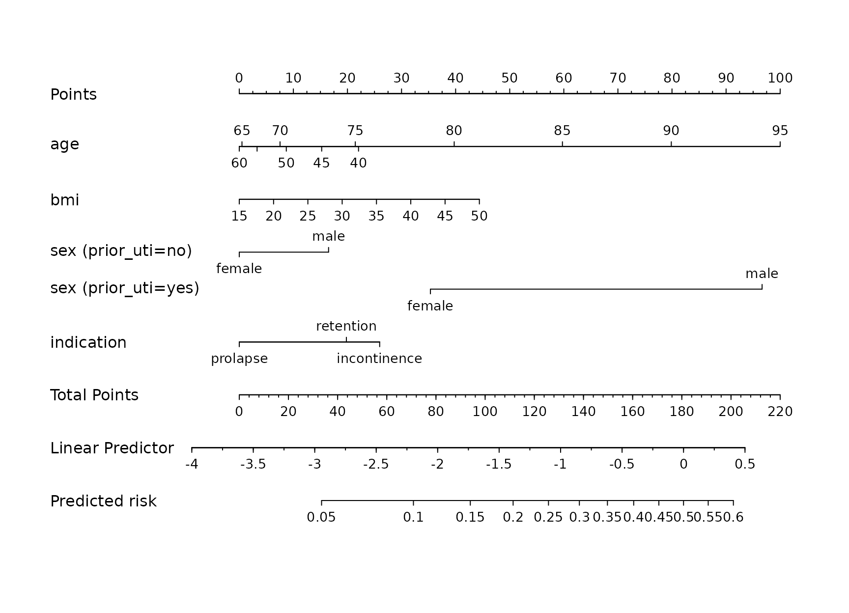

The interaction makes rms emit mutually exclusive axes, so a predictor’s ticks have to be gathered across axes rather than read off one:

mysterymodel:::mm_axis_names(nom$nomogram)
#> [1] "age"                 "bmi"                 "sex (prior_uti=no)" 
#> [4] "sex (prior_uti=yes)" "indication"
str(mysterymodel:::mm_axis_values(nom$nomogram, plan$D$predictors))
#> List of 5
#>  $ age       : int [1:12] 40 45 50 55 60 65 70 75 80 85 ...
#>  $ bmi       : int [1:8] 15 20 25 30 35 40 45 50
#>  $ sex       : chr [1:2] "female" "male"
#>  $ prior_uti : chr [1:2] "no" "yes"
#>  $ indication: chr [1:3] "incontinence" "prolapse" "retention"

Every tick of every axis, exercised:

profiles <- mysterymodel:::mm_tick_profiles(nom$nomogram, fits$D)
c(profiles = nrow(profiles), checked = nom$profiles_checked)
#> profiles  checked 
#>       27       27
head(profiles, 3)
#>   age bmi    sex prior_uti   indication
#> 1  40  15 female        no incontinence
#> 2  45  15 female        no incontinence
#> 3  50  15 female        no incontinence

flattened <- profiles
flattened$indication <- as.character(flattened$indication)
restored <- mysterymodel:::mm_restore_levels(flattened, fits$D$schema)
identical(levels(restored$indication),
          fits$D$schema$predictors$indication$levels)
#> [1] TRUE

At a tabulated tick, summing the points by hand and converting on the printed axis reproduces the model exactly. This is the agreement mm_nomogram() asserts, done one profile at a time:

on_tick <- profiles[6, , drop = FALSE]
total <- unname(mysterymodel:::mm_nomogram_points(nom$nomogram, on_tick))
lp <- mysterymodel:::mm_total_to_lp(nom$nomogram, total)

c(points = total, linear_predictor = lp, risk_from_axis = plogis(lp),
  risk_read_back = unname(
    mysterymodel:::mm_nomogram_risk(nom$nomogram, on_tick)),
  risk_from_model = mm_predict(fits$D, on_tick)$.pred)
#>           points linear_predictor   risk_from_axis   risk_read_back 
#>      26.45594560      -3.08480098       0.04373857       0.04373857 
#>  risk_from_model 
#>       0.04373857

A real patient does not land on a tick. Between ticks the spline curves and the straight line between printed values does not, so the reading carries the axis’s own resolution error:

patient <- data.frame(
  age = 71, bmi = 33.5,
  sex = factor("male", levels = fits$D$schema$predictors$sex$levels),
  prior_uti = factor("yes",
                     levels = fits$D$schema$predictors$prior_uti$levels),
  indication = factor("retention",
                      levels = fits$D$schema$predictors$indication$levels))

read_off <- unname(mysterymodel:::mm_nomogram_risk(nom$nomogram, patient))
from_model <- mm_predict(fits$D, patient)$.pred

c(read_off = read_off, from_model = from_model,
  gap = abs(read_off - from_model),
  worst_between_ticks = nom$reading_error)
#>            read_off          from_model                 gap worst_between_ticks 
#>         0.352262742         0.350086748         0.002175994         0.004841919

This patient is off-tick in age and BMI at once, which is the case a one-predictor-at-a-time probe never visits: points are additive, so a reading accumulates both axes’ interpolation errors. reading_error is a bound rather than a probe for that reason, and the gap above sits under it.

ticks <- mysterymodel:::mm_axis_values(nom$nomogram, plan$D$predictors)
set.seed(8)
anywhere <- data.frame(
  age = runif(300, min(ticks$age), max(ticks$age)),
  bmi = runif(300, min(ticks$bmi), max(ticks$bmi)),
  sex = factor(sample(fits$D$schema$predictors$sex$levels, 300, TRUE),
               levels = fits$D$schema$predictors$sex$levels),
  prior_uti = factor(sample(fits$D$schema$predictors$prior_uti$levels,
                            300, TRUE),
                     levels = fits$D$schema$predictors$prior_uti$levels),
  indication = factor(sample(fits$D$schema$predictors$indication$levels,
                             300, TRUE),
                      levels = fits$D$schema$predictors$indication$levels))

anywhere_read <- vapply(seq_len(nrow(anywhere)), function(i) unname(
  mysterymodel:::mm_nomogram_risk(nom$nomogram,
                                  anywhere[i, , drop = FALSE])), numeric(1))
worst_joint <- max(abs(anywhere_read - mm_predict(fits$D, anywhere)$.pred))
c(bound = nom$reading_error, worst_over_300_joint_profiles = worst_joint,
  bound_holds = nom$reading_error >= worst_joint)
#>                         bound worst_over_300_joint_profiles 
#>                   0.004841919                   0.004127436 
#>                   bound_holds 
#>                   1.000000000

Three hundred profiles drawn anywhere inside the printed axes, and none of them beats the bound. That is the property being claimed, and it comes from the error decomposing rather than from having looked in enough places: the discrepancy is the points-to-lp slope times the sum of each axis’s own interpolation error, each of which is zero at its own ticks, so the extremes of the sum are the sums of the extremes.

nom$reading_error_by_axis
#>                lo         hi
#> age -6.661338e-16 0.01936783
#> bmi -6.661338e-16 0.00000000

Which says where the coarseness is, and so which axis would need more ticks. The gap belongs to every printed nomogram and to every clinician reading one. What this package adds is a number that cannot be exceeded by a reading rather than one that happened not to be.

totals <- vapply(seq_len(nrow(profiles)), function(i) unname(
  mysterymodel:::mm_nomogram_points(nom$nomogram,
                                    profiles[i, , drop = FALSE])), numeric(1))
c(lowest_profile = min(totals), axis_starts = min(nom$nomogram$lp$x),
  off_scale_profiles = sum(mysterymodel:::mm_off_axis(nom$nomogram, totals)),
  reported = nom$off_axis)
#>     lowest_profile        axis_starts off_scale_profiles           reported 
#>           22.04708          -19.30386            0.00000            0.00000

direct <- mysterymodel:::mm_reading_error(nom$nomogram, fits$D)
c(between_ticks = direct$bound, lp_scale = direct$lp,
  reported = nom$reading_error, at_ticks = nom$worst_disagreement)
#> between_ticks      lp_scale      reported      at_ticks 
#>  4.841919e-03  1.936783e-02  4.841919e-03  5.551115e-17

exported <- mysterymodel:::mm_nomogram_export(
  nom$nomogram, figures, "worked-example", width = 13, height = 9)
#> wrote 3 nomogram file(s): /tmp/Rtmp1Zg5XE/worked-example/worked-example_nomogram.pdf, /tmp/Rtmp1Zg5XE/worked-example/worked-example_nomogram.svg, /tmp/Rtmp1Zg5XE/worked-example/worked-example_nomogram.png
basename(exported)
#> [1] "worked-example_nomogram.pdf" "worked-example_nomogram.svg"
#> [3] "worked-example_nomogram.png"
basename(nom$files)
#> [1] "uds-d_nomogram.pdf" "uds-d_nomogram.svg" "uds-d_nomogram.png"

10. One patient at a time

ward <- data.frame(
  age        = c(58, 71, 104),
  bmi        = c(24.0, 33.5, 28.0),
  sex        = factor(c("female", "male", "female"),
                      levels = fits$D$schema$predictors$sex$levels),
  prior_uti  = factor(c("no", "yes", "no"),
                      levels = fits$D$schema$predictors$prior_uti$levels),
  indication = factor(c("incontinence", "retention", "prolapse"),
                      levels = fits$D$schema$predictors$indication$levels))

mm_predict(fits$D, ward)
#>        .pred .extrapolated
#> 1 0.05485948         FALSE
#> 2 0.35008675         FALSE
#> 3 0.36364259          TRUE

unseen <- ward[1, ]
unseen$indication <- factor(
  "urgency", levels = c(levels(ward$indication), "urgency"))
mm_predict(fits$D, unseen)
#> Error:
#> ! `indication` has level(s) the model never saw: urgency. Known: incontinence, prolapse, retention. A level absent from development cannot be scored.

incomplete <- ward[1, ]
incomplete$bmi <- NA
mm_predict(fits$D, incomplete)
#> Error:
#> ! 1 row(s) have a missing predictor. A complete-data model cannot score them. Impute first, or pass on_missing = "na".

mm_predict(fits$D, incomplete, on_missing = "na")
#>   .pred .extrapolated
#> 1    NA         FALSE

11. Provenance

do.call(rbind, lapply(names(fits), function(k) data.frame(
  analysis = k,
  coefficients = substr(fits[[k]]$fingerprint, 1, 12),
  development = substr(fits[[k]]$development, 1, 12),
  validation_matches = identical(checked[[k]]$fingerprint,
                                 fits[[k]]$fingerprint))))
#>   analysis coefficients  development validation_matches
#> 1        A 20486eeb8ce2 c9552f752ad9               TRUE
#> 2        B b40edbe891b8 c9552f752ad9               TRUE
#> 3        C 93ca893c5644 d3e0c5b952e9               TRUE
#> 4        D 3b00d7880d0b a97f8dd9ff7e               TRUE

A and B share a development sample and differ in shape, so their coefficient fingerprints differ and their development fingerprints agree. D reserved rows, so both of its fingerprints stand alone.

12. Coverage, proved rather than claimed

exported_fns <- getNamespaceExports("mysterymodel")
everything <- ls(asNamespace("mysterymodel"))
everything <- everything[grepl("^mm_", everything)]

source_text <- tryCatch(
  readLines(knitr::current_input()), error = function(e) character(0))
used <- vapply(everything, function(fn)
  any(grepl(paste0("\\b", fn, "\\b"), source_text)), logical(1))

c(functions = length(everything),
  exported = length(intersect(everything, exported_fns)),
  used_here = sum(used))
#> functions  exported used_here 
#>        55        10        40
sort(everything[!used])
#>  [1] "mm_anova_block"           "mm_candidate_pairs"      
#>  [3] "mm_draw_splines"          "mm_exclusive_axes"       
#>  [5] "mm_interaction_health"    "mm_interaction_rank"     
#>  [7] "mm_interaction_support"   "mm_matrix_rank"          
#>  [9] "mm_min_resamples"         "mm_no_corrected_interval"
#> [11] "mm_no_information"        "mm_parameter_budget"     
#> [13] "mm_reference_profile"     "mm_undrawable_blocks"    
#> [15] "mm_unfittable_ordered"

The ones it does not reach are helpers whose results are already on the page rather than capabilities going untested: the four-fifths resample floor and the no-information Brier appear in the validation notes above, the sentence about a corrected c-statistic’s missing interval is printed in those notes verbatim, and the rank and support machinery behind the interaction screen is summarised in its own columns. Naming them is the point of the chunk, and the list is printed rather than described so it cannot quietly go stale.

methods_used <- c("print.mm_project", "print.mm_cohort", "print.mm_eda",
                  "print.mm_model", "print.mm_adequacy",
                  "print.mm_validation", "print.mm_nomogram")
vapply(methods_used, function(m) any(grepl(
  sub("^print\\.", "", m), vapply(list(plan$D, eligible, described, fits$D,
                                       fits$C$adequacy, checked$D, nom),
                                  function(x) class(x)[1], character(1)))),
  logical(1))
#>    print.mm_project     print.mm_cohort        print.mm_eda      print.mm_model 
#>                TRUE                TRUE                TRUE                TRUE 
#>   print.mm_adequacy print.mm_validation   print.mm_nomogram 
#>                TRUE                TRUE                TRUE

Everything above ran on synthetic data. The package carries none of its own, and the one number worth distrusting in the whole article is the held-out column: one temporal split of one cohort, scored once, which says nothing about a different hospital in a different year.